1.5. Example: Solving inviscid Burgers’ equation using IVP interface

Here we demonstrate how to use the ivp (initial-value problem for ordinary differential equations, that is, time integration) interface with Python bindings to solve the following problem based on the inviscid Burgers’ equation:

\[\begin{split} \begin{align} u_t + \left(\frac{u^2}{2}\right)_x &= 0, \quad x \in [0, 2], \quad t \in [0, 2], \\ u(0, x) &= 0.5 - 0.25 \sin(\pi x), \\ u(t, 0) &= u(t, 2) \end{align} \end{split}\]

This is one of the most famous nonlinear hyperbolic equations with the property that some initial conditions, although smooth, can lead to jump discontinuities in the solution at some final time. These jump discontinuities are called shock waves. The initial condition that we choose is exactly of this type, so that at the final time \(T = 2\) the solution develops a shock wave.

To deal with such properties, special numerical methods are used that smooth the discontinuity a bit so that the computation process remains stable.

Also, it is common to use special time integration schemes with an upper bound on the time step, also to keep things numerically stable.

Here, instead of using such special methods for time integration, we will use adaptive integration. To facilitate this, we will convert the partial differential equation into a system of ODEs:

\[ \frac{du_i}{dt} = -0.5 \frac{\partial u_i^2}{\partial x} \]

which is commonly discretized in space (the right-hand side) in the following way:

(1.5.1)\[\frac{du_i}{dt} = - \frac{\hat f(u_{i + 1/2}) - \hat f(u_{i - 1/2})}{\Delta x},\]

where \(f = 0.5 u^2\) and \(\hat f\) is an approximation of \(f\). There are different ways of approximating \(f\), we will use one of the simplest just for the sake of a demonstration.

The code goes like this:

impl = "scipy_ode_dopri5"
problem = BurgersEquationProblem(N=101)
s = IVP(impl)
s.set_initial_value(problem.u, problem.t0)
s.set_rhs_fn(problem.compute_rhs)

Here we use an auxiliary class BurgersEquationProblem that handles details of the computations of the initial conditions and the right hand side of the equation :eqref:. The details of the actual computations are somewhat irrelevant as the most important thing here is that we instantiate the IVP interface, with a given implementation that we want to use, then we invoke the set_initial_value method with the actual initial conditions, and the set_rhs_fn method that takes a callback that evaluates the right-hand side of the system Eq. 1.5.1. Important here is that callback has a signature rhs(t, u, udot), where t is time to which we want to integrate currently, u is the ndarray with current values of the ODE system solution vector, and udot is ndarray to which computed right-hand side is written.

Once we set the details, we can do actual integrations at given time points:

times = np.linspace(problem.t0, problem.tfinal, num=11)

soln = [y0]
for t in times[1:]:
s.integrate(t)
print(f"{t:.3f} {s.y[0]:.6f}")
soln.append(s.y)

and plot the results:

import matplotlib.pyplot as plt
plt.plot(problem.x, soln[0], '--', label="Initial condition")
plt.plot(problem.x, soln[-1], '-', label="Final solution")
plt.legend(loc="best")
plt.savefig("examples_burgers_eq.pdf")

The actual solution at the final time \(T = 2\) and the initial condition are shown on the figure.

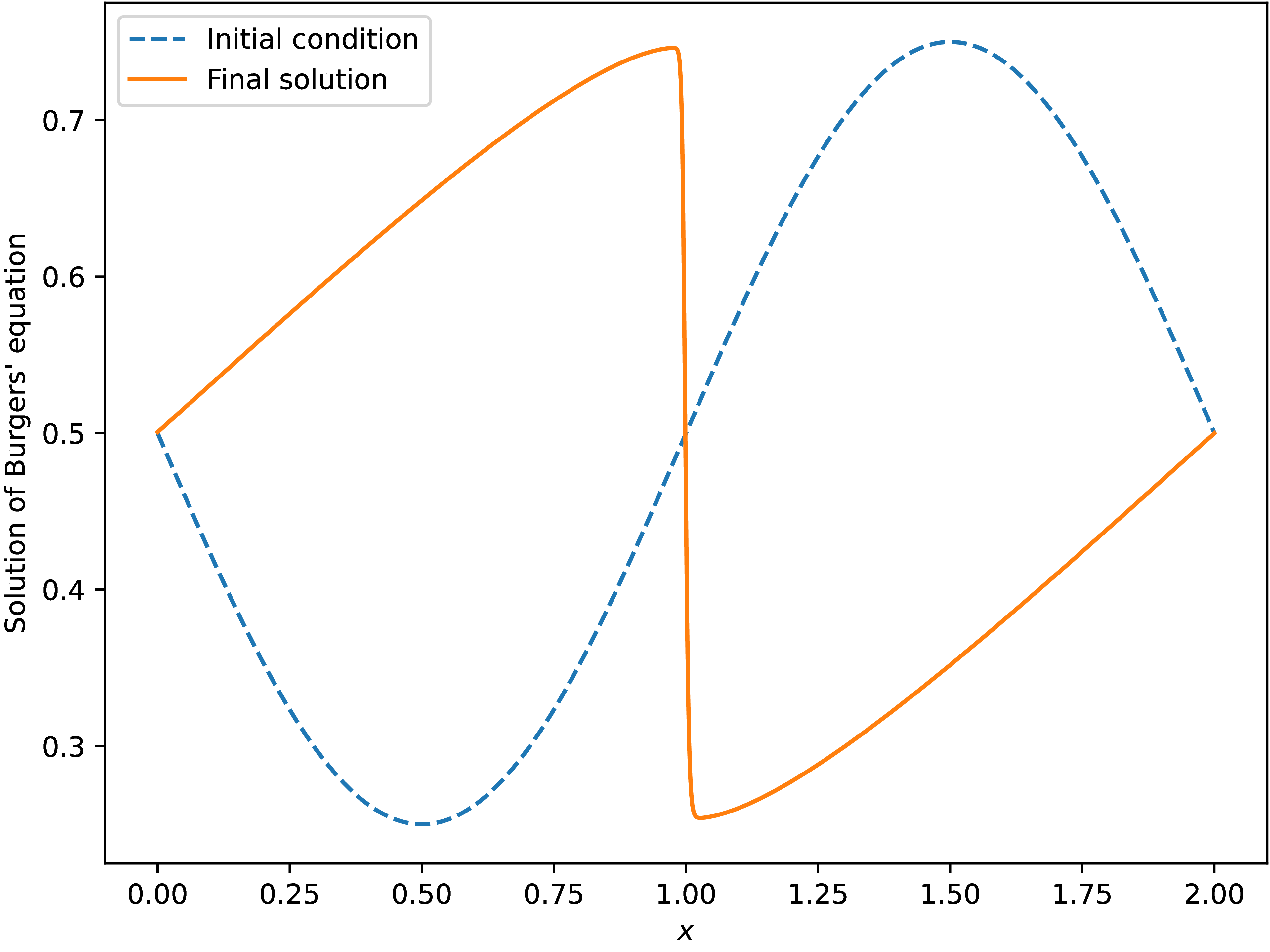
Fig. 1.5.1 Numerical solution of the problem for Burgers’ equation via IVP interface of Open InterFaces using scipy_ode_dopri5 implementation.