1.4. Example: Solve van der Pol equation using C¶

In this example, we use Open Interfaces from C to solve Van der Pol equation:

\[ \frac{\mathrm d^2 x}{\mathrm d t^2} - \mu \left( 1 - x^{2} \right) \frac{\mathrm d x}{\mathrm d t} + x = 0, \quad x(0) = 2\]

with parameter $\mu = 1000$, on time interval $t \in [0, 3000]$. Note that such a high value of $\mu$ makes the system stiff, in a sense that it exhibits both fast and slow dynamics and explicit methods for solving initial-value problems are not efficient for such systems as they require very small time steps to maintain stability.

To solve this second-order ordinary differential equation, we first rewrite it as a system of two first-order ordinary differential equations:

\[\begin{split} \frac{\mathrm d u_1}{\mathrm d t} &= u_2, \quad \\ \frac{\mathrm d u_2}{\mathrm d t} &= \mu (1 - u_1^2) u_2 - u_1, \quad \\ u_1(0) &= 2, \quad \\ u_2(0) &= 0,\end{split}\]

where $u_1 = x$ and $u_2 = \frac{\mathrm d x}{\mathrm d t}$.

We implement the right-hand side of this system in the class VdPEquationProblem to avoid passing parameter $\mu$ to the function that computes the right-hand side:

int
rhs(double t, OIFArrayF64 *y, OIFArrayF64 *ydot, void *user_data)
{
    (void)t;  // Unused
    double mu = *(double *)user_data;
    ydot->data[0] = y->data[1];
    ydot->data[1] = mu * (1 - y->data[0] * y->data[0]) * y->data[1] - y->data[0];

    return 0;
}

Note that the function rhs has a signature defined by the IVP interface, such as it accepts time t, current state y, and computes the time derivative ydot at the current state and time. The user_data pointer is used to pass additional data to the function, in our case, parameter mu. Also, it returns 0 at the end to indicate successful computation.

Having defined the right-hand side of the system, we can set other parameters of the initial-value problem: namely, time span and the problem parameter:

    double t0 = 0.0;
    double t_final = 3000;
    double mu = 1e3; // Stiffness parameter.

After that, we use the OIFArrayF64 structure to define two arrays: one for the initial state y0 and another one for the solution y at current time:

    const int N = 2;  // Number of equations in the system.
    OIFArrayF64 *y0 = oif_create_array_f64(1, (intptr_t[1]){N});
    OIFArrayF64 *y = oif_create_array_f64(1, (intptr_t[1]){N});

and then set the initial state:

    y0->data[0] = 2.0; // u1(0) = 2
    y0->data[1] = 0.0; // u2(0) = 0

After that we load an implementation of the IVP interface. For example, we can use the implementation based on SciPy library:

solver = IVP("scipy_ode")
    ImplHandle implh = oif_load_impl("ivp", impl, 1, 0);

Pass the initial condition:

    status = oif_ivp_set_initial_value(implh, y0, t0);

Set the user data (parameter mu in our case)

    status = oif_ivp_set_user_data(implh, &mu);

Set the right-hand side function: status = oif_ivp_set_rhs_fn(implh, rhs);

and set the required tolerances:
```c
    status = oif_ivp_set_tolerances(implh, 1e-8, 1e-12);

We also define a constant Nt for number of time steps, variable dt for a time step, and two additional arrays to hold the solution time series:

    const int Nt = 501;
    double dt = (t_final - t0) / (Nt - 1);

    OIFArrayF64 *times = oif_create_array_f64(1, (intptr_t[1]){Nt});
    OIFArrayF64 *solution = oif_create_array_f64(1, (intptr_t[1]){Nt});
    times->data[0] = t0;
    solution->data[0] = y0->data[0];

The integration loop is as follows:

    for (int i = 1; i < Nt; ++i) {
        double t = t0 + i * dt;
        if (t > t_final) {
            t = t_final;
        }
        oif_ivp_integrate(implh, t, y);
        times->data[i] = t;
        solution->data[i] = y->data[0];
    }

If we run the code, we receive the following error message:

/home/user/sw/miniforge3/envs/open-interfaces/lib/python3.13/site-packages/scipy/integrate/_ode.py:438: UserWarning: dopri5: larger nsteps is needed
  self._y, self.t = mth(self.f, self.jac or (lambda: None),
Traceback (most recent call last):
  File "/home/dima/Work/um02-open-interfaces/lang_python/oif_impl/openinterfaces/_impl/ivp/scipy_ode/scipy_ode.py", line 62, in integrate
    assert self.s.successful()
           ~~~~~~~~~~~~~~~~~^^
AssertionError
[bridge_python] Call failed
[dispatch] ERROR: During execution of the function 'ivp::integrate' an error occurred

due to the fact that the default maximum number of steps is not allowed to solve this stiff problem.

Even if we increase the maximum number of steps allowed:

    oif_config_dict_add_int(dict, "nsteps", 100000);
    status = oif_ivp_set_integrator(implh, "dopri5", dict);

and integrate again, we receive the same error message.

Even, if we switch to another solver available in SciPy, for example, vode with bdf method:

   oif_config_dict_add_str(dict, "method", "bdf");
   status = oif_ivp_set_integrator(implh, "vode", dict);

we still receive the same error message due to the stiffness of the problem.

We have to increase the maximum number of steps allowed for the vode solver to a high value, for example, 40 000 steps:

oif_config_dict_add_str(dict, "method", "bdf");
oif_config_dict_add_int(dict, "nsteps", 40000);
status = oif_ivp_set_integrator(implh, "vode", dict);

and only then, the solver is able to solve the problem and we arrive at the solution Figure Fig. 1.4.1, although integration takes a while (about 8 seconds in our experiments).

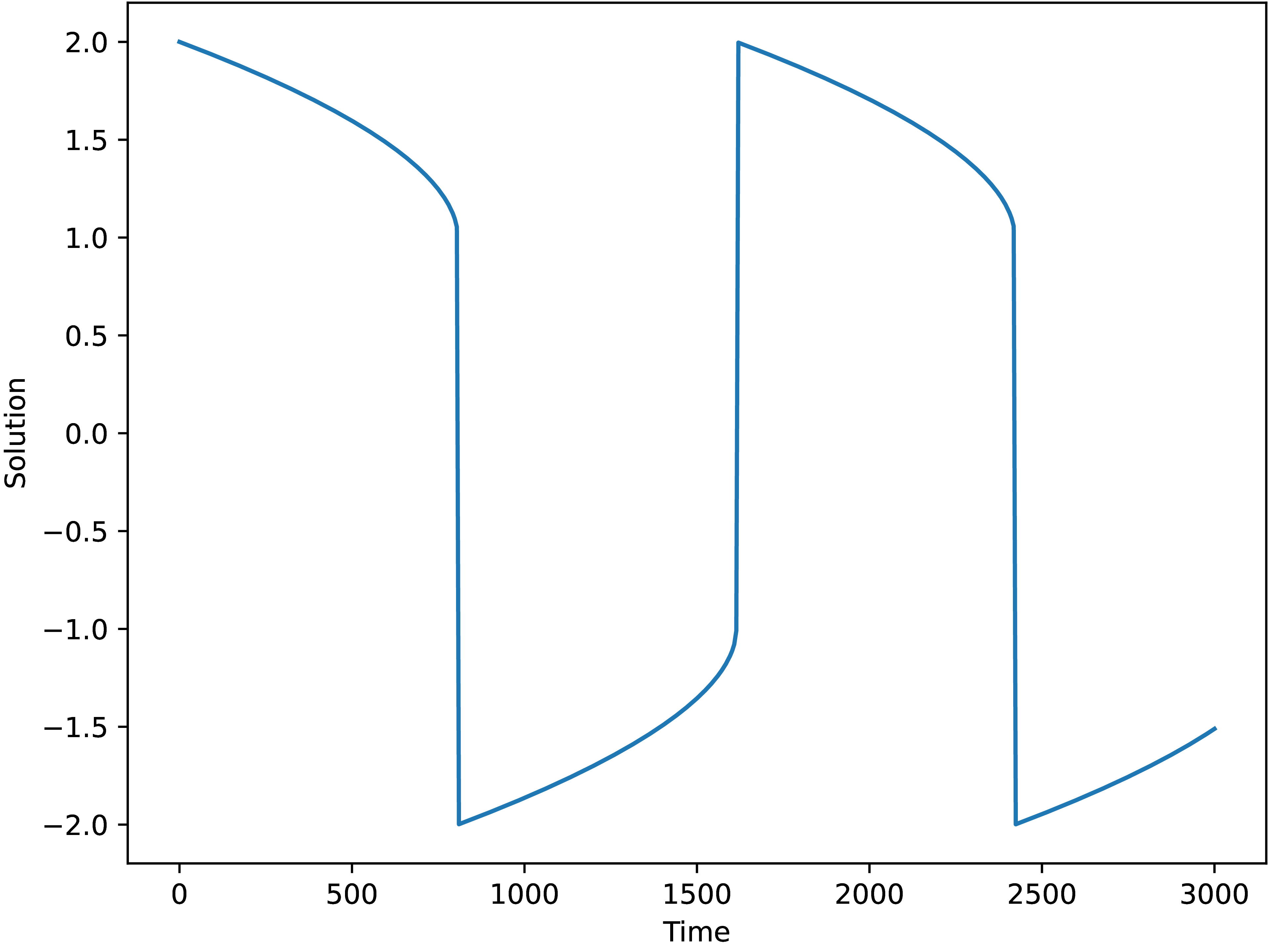
Fig. 1.4.1 Solution of the Van der Pol equation with $mu=1000$ using `scipy_ode` with the `vode` integrator.¶

Finally, we try to use other implementations of the IVP interface, for example, Rosenbrok23 integrator from the OrdinaryDiffEq.jl Julia package, which in Open Interfaces is available via the jl_diffeq implementation:

ImplHandle implh = oif_load_impl("ivp", "jl_diffeq", 1, 0);
oif_ivp_set_integrator(implh, "Rosenbrock23", NULL);

(here we replace Automatic Differentiation with Forward Differencing by supplying an integration option autodiff=False; we are working currently on enabling use of Automatic Differentiation in jl_diffeq). Running the code with this implementation, we arrive at the solution quickly (about 1 second), see Fig. 1.4.2. One can see that the solution is the same as the one obtained with the vode solver from SciPy, Fig. 1.4.1.

Solution of the Van der Pol equation with mu=1000 using the `jl_diffeq` implementation with the `Rosenbrok23` integrator. — Fig. 1.4.2 Solution of the Van der Pol equation with mu=1000 using `jl_diffeq` implementation with the `Rosenbrok23` integrator.¶

The full code of this example is available in the examples/call_ivp_from_c_vdp_eq.c and can be run as follows:

build/xamples/examples/call_ivp_from_c_call_ivp_from_c_vdp_eq.c [implementation] [integrator]

where the implementation and integrator arguments the following pairs:

scipy_ode and dopri5,
scipy_ode and dopri5-100k,
scipy_ode and vode,
scipy_ode and vode-40k,
jl_diffeq and rosenbrock23.

At the end of the computations, if they are successful, the resultant solution is written to a file solution.txt that can be plotted using Python, for example, as follows:

import matplotlib.pyplot as plt
import numpy as np

t, u = np.loadtxt("solution.txt")

plt.figure()
plt.plot(t, u, "-", label=r"y(t)")
plt.show()