5.8. 2024-03-12 IVP CVODE performance study

This technical note documents performance study based on integration of the 2D Gray–Scott reaction-diffusion system using IVP interface for time integration with Sundials CVODE solver. The user code is implemented in Python, hence the performance base is direct bindings of the CVODE solver via scikits.odes Python package.

5.9. Details

We solve 2D Gray–Scott reaction-diffusion system:

(5.9.1)\[\begin{split}\begin{align} \frac{\partial u}{\partial t} = d_u \nabla^2 u - u v^2 + F (1 - u), \\ \frac{\partial v}{\partial t} = d_v \nabla^2 v + u v^2 - (F + k) v \end{align}\end{split}\]

with periodic boundary conditions on the domain \([-2.5; 2.5]^2\) with initial condition given by \(u = 1\), \(v = 0\) everywhere in the domain, except a square of \(40 \times 40\) grid points centered in the center of the domain, which was set to \(u = 0.5 + U(0; 0.1)\) and \(v = 0.25 + U(0; 0.1)\), where \(U\) is a uniform distribution.

The system is evolved to time \(T = 100\) with time step 1. The resolution \(N\) in \(x\) and \(y\) directions was the same with \(N \in {64, 128, 256, 512}\). Parameters of the problem are set to values \(F = 0.055\), \(k = 0.062\), \(d_u = \num{2e-5}\), \(d_v = \num{e-5}\).

5.9.1. Procedure

We analyze performance using command

python examples/compare_performance_ivp_burgers_eq.py all --n_runs 3

which solves the problem Eq. 5.9.1 via Open Interfaces’s IVP interface with Sundials CVODE solver and via direct binding to this solver from scikit.odes version 2.7.0 package.

Both implementations are linked to the same version of compiled Sundials 6.7.

Non-default parameters for CVODE are: relative and absolute tolerance \(10^{-15}\), no linear solver, fixed point nonlinear solver.

In the above command --n_runs 3 means that for each \(N\) and implementation, the same computations were done three times, so that the results below are averaged, and the standard error of the mean is reported.

5.9.2. Normalized performance results

Figure shows the normalized runtimes (with respect to the “native” results, that is, direct invocation of the ode class from scikits.odes).

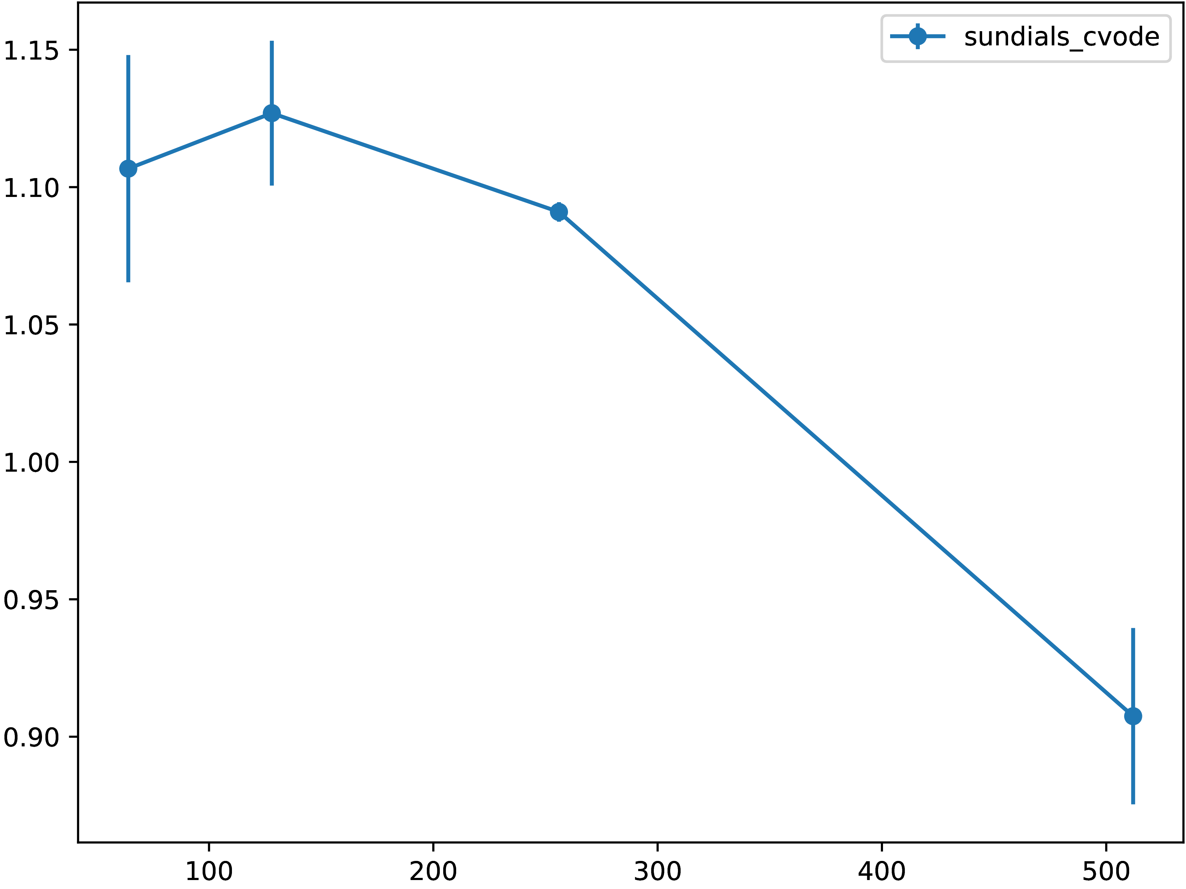
Fig. 5.9.1 Normalized runtime relative to the “native” code executation of directly calling scikits.odes from Python for different grid resolutions.

We can see from the figure that for small resolutions we have about 10% performance penalty, while for larger resolutions the Open Interfaces implementation actually outperforms the result obtained via direct Python-to-C bindings of scikits.odes.

5.9.3. Quantitative data

The following table shows numbers behind the previous figure

           N                  64                128               256               512
sundials_cvode             0.40   0.01       1.81   0.01      10.51   0.07      75.79   0.39
native_sundials_cvode      0.42   0.03       1.90   0.04      11.02   0.26      76.63   0.75